Machine Learning
Data Collection
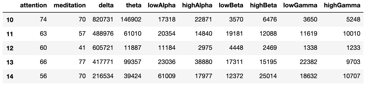
The sensor we use is the Mindwave Mobile 2 EEG headset from NeuroSky, which costs $99. When requested, the headset sends 1 reading of data every 1 second, which includes the following values: attention (user’s attention level measured by the headset), meditation (user’s relaxation level measured by the headset), delta, theta, low alpha, high alpha, low beta, high beta, low gamma, and high gamma. The last 8 values in the data are brainwave bands values, which we use in our emotion classification algorithm. The first 2 values are obtained from the headset’s own algorithm (not raw brainwave values) and therefore are not used in our algorithm. A sample of the sensor reading is shown below.
Our training data is collected from 3 participants, 2 males and 1 female. The positive/negative emotion data are collected by asking the participants to attentively watch funny or sad Youtube videos in a quiet room without any distraction. The emotional self-assessment of the participants after watching the video is also taken into account, and only the data assessed as truly positive or negative is used in training. A total of 4800 seconds of data is collected for training, in which about 45% is positive and 55% is negative.
Data Preprocessing
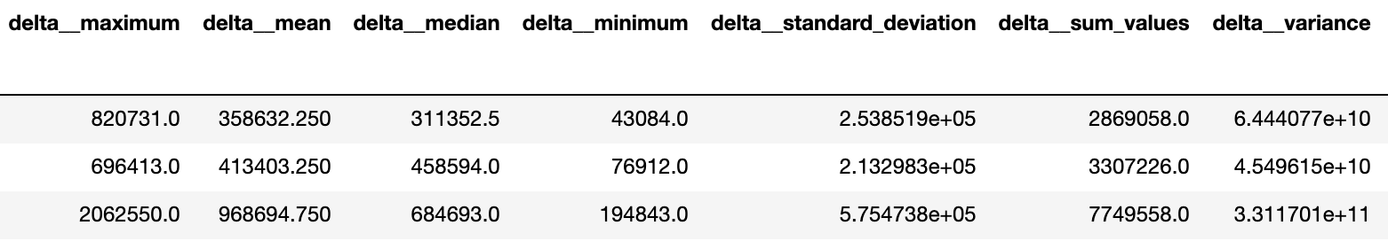
After the training data is collected, cleaning of the data is done to remove missing values and zero values from the data. The cleaned data are then divided into 8-second sequences in order to extract time series features. Therefore, the sequences each has 8 rows corresponding to 8 seconds of readings, and 8 columns corresponding to the 8 brainwave band values. To extract features from the sequences, the “tsfresh” package in Python is used, and 64 features are extracted from each sequence; thus, each sequence is transformed into 1 row of data with 64 columns. A sample of the data after feature extraction is shown below.
The data after feature extraction is then used as training data for the machine learning classifier models.
Model Selection
A wide variety of machine learning classifier models have been used in previous research papers, so experiments had to be done for us to pick the best model. Using Python and Scikit-learn, we initially tried 10 classifier, including K nearest neighbors (KNN), SVM, Decision Tree, Random Forest, AdaBoost, Gradient Boosting, Gaussian Naive Bayes, Linear Discriminant Analysis (LDA), Quadratic Discriminant Analysis, and XGBoost (XGB).
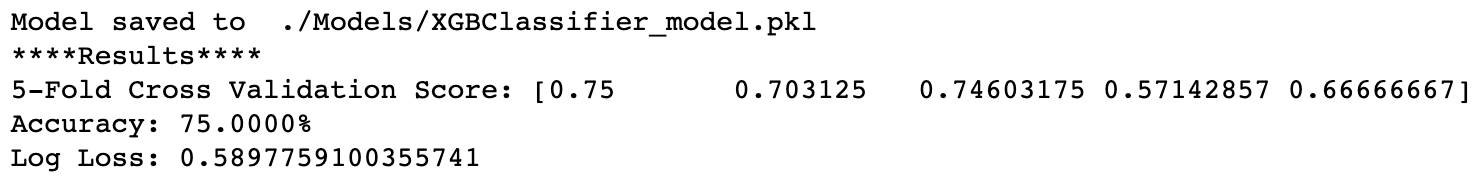
After calculating the 5-fold cross validation score for each of the models, we observed that 3 of the models had poor performance on all datasets, while the other 7 models had good performance on some dataset but the performances were not stable. Therefore, we decided to build a voting ensemble with these 7 models to balance out the weaknesses of each model. The experiment result of the XGB classifier is shown below as an example.
After calculating the 5-fold cross validation score for each of the models, we observed that 3 of the models had poor performance on all datasets, while the other 7 models had good performance on some dataset but the performances were not stable. Therefore, we decided to build a voting ensemble with these 7 models to balance out the weaknesses of each model. The experiment result of the XGB classifier is shown below as an example.
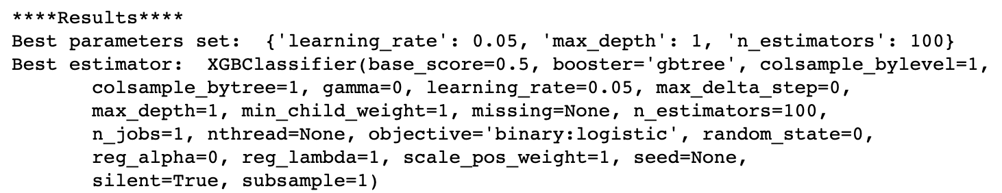
The 7 models we selected to build the voting ensemble are the following: KNN, Decision Tree, Random Forest, AdaBoost, Gradient Boosting, LDA, and XGB. To further increase the accuracy, we used Grid Search to find the best hyperparameter set for each of the 7 models. The Grid Search result of the XGB classifier is shown below as an example.
After training the 7 models with best hyperparameter sets, we saved the trained models and used them to build the voting ensemble, which is applied in our final system.
